
To add a dollar sign in Google Sheets, simply type a dollar sign ($) before the number or cell reference. We will discuss the steps to easily add a dollar sign in Google Sheets and ensure that it appears consistently in your data.
Whether you’re working with financial data or need to format currency values, adding a dollar sign can help provide clarity and improve readability. By following these straightforward instructions, you’ll be able to effectively display currency values in your Google Sheets, making them easier to understand and analyze.
Let’s dive into the details and learn how to add a dollar sign in Google Sheets.

Credit: www.ablebits.com
Understanding Currency Formatting
When working with financial data in Google Sheets, it is crucial to understand currency formatting. By applying currency formatting to your cells, you can display numbers in a chosen currency format, complete with symbols, decimal places, and thousands separators. This not only improves the visual representation of your data but also ensures accurate calculations and easy readability.
What Is Currency Formatting?
Currency formatting in Google Sheets allows you to customize the appearance of your numbers and represent them as monetary values. It involves adding a specific currency symbol, deciding on the number of decimal places, and including thousands separators to enhance the readability of your data.
Apart from the dollar sign ($), you can choose from a variety of currency symbols such as euros (€), pounds (£), yen (¥), or any other currency symbol depending on your needs. By applying currency formatting, you can ensure consistency and clarity in presenting your financial information.
Why Is Currency Formatting Important?
Currency formatting is essential for several reasons:
- Clear representation: By using currency symbols and specific decimal places, you can make your numbers more comprehensible for your audience. It enables them to quickly identify the currency and understand the magnitude of the amounts.
- Accurate calculations: Currency formatting ensures correct calculations when performing financial operations. By specifying the number of decimal places, you can avoid rounding errors and maintain precision in your calculations.
- Consistency: By applying currency formatting throughout your spreadsheet, you maintain consistency in representing financial values. This consistency enhances the overall look and readability of your data.
- Localization: Currency formatting allows you to adapt your spreadsheet to different regions and countries with ease. You can effortlessly switch between currency symbols and formats to cater to the needs of your target audience or stakeholders.
Understanding and utilizing currency formatting in Google Sheets is an important skill for anyone handling financial data. By presenting your numbers accurately and clearly, you can ensure effective communication of your financial insights.


Credit: www.amazon.com
Adding Dollar Sign In Google Sheets
Adding a dollar sign ($) in Google Sheets can be useful when you are working with financial data or currency values. The dollar sign is a symbol that represents a specific currency and is commonly used in financial contexts. In this article, we will explore three different methods for adding a dollar sign in Google Sheets.
Method 1: Using The Format Menu
To add a dollar sign in Google Sheets using the Format menu, follow these steps:
- First, select the cell or range of cells where you want to add the dollar sign.
- Next, navigate to the “Format” menu in the toolbar at the top of the screen.
- In the dropdown menu, click on “Number”.
- A submenu will appear. Select “Currency” from the options.
- In the currency dropdown, choose the currency symbol you want to use (in this case, the dollar sign).
- Optionally, you can customize the decimal places and other formatting options.
- Click “Apply” to add the dollar sign to the selected cells.
Method 2: Using The Dollar Sign Button
Google Sheets also provides a convenient button for adding a dollar sign to cells. Here’s how you can use it:
- Select the cell or range of cells where you want to insert the dollar sign.
- Locate the “Number format” dropdown menu in the toolbar.
- Click on the button shaped like a dollar sign ($).
- The dollar sign will be applied to the selected cells immediately.
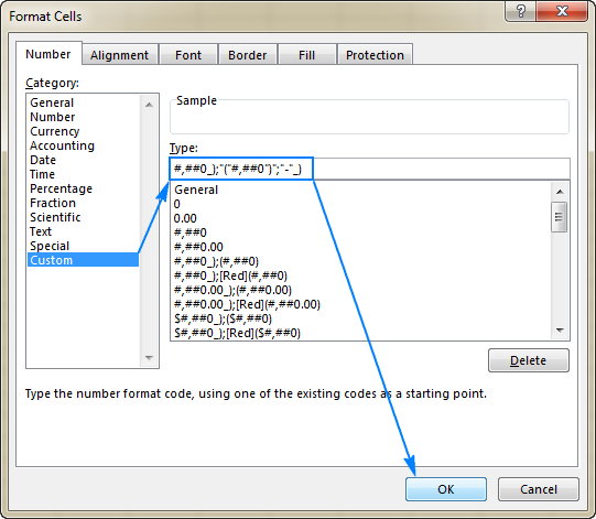
Method 3: Using Custom Number Formatting
If you need more control over the appearance of the dollar sign, you can use custom number formatting. Follow these steps:
- Select the cell or range of cells where you want to add the dollar sign.
- Right-click on the selected cells and choose “Format cells” from the context menu.
- In the “Number” tab, select “More formats” and then choose “Custom number format”.
- In the input box, enter the desired format code, including the dollar sign.
- For example, to display a dollar sign before the number, you can use “$0.00”.
- Click “Apply” to apply the custom number format to the selected cells.
Mastering Currency Formatting
Formatting numbers as currency is crucial when working with financial data or creating invoices in Google Sheets. Understanding how to add a dollar sign and control decimal places can greatly enhance the clarity and professionalism of your spreadsheets. In this guide, we will explore the various techniques to master currency formatting in Google Sheets.
Formatting Multiple Cells At Once
When working with large sets of data in Google Sheets, manually formatting each cell individually can be time-consuming and tedious. Fortunately, you can quickly format multiple cells at once using a simple selection.
To format multiple cells, follow these easy steps:
- Highlight the range of cells you want to format.
- Right-click on the selected range and choose “Format cells” from the context menu.
- In the “Format cells” dialog box, navigate to the “Number” tab.
- Select the “Currency” category and choose your desired options, such as decimal places and currency symbol.
- Click “Apply” to apply the currency formatting to the selected range of cells.
Changing The Currency Symbol
Google Sheets allows you to easily change the currency symbol to match the currency you are working with. Whether it’s the dollar sign ($), euro symbol (€), pound sterling (£), or any other currency symbol, you can personalize the currency formatting to suit your needs.
To change the currency symbol, follow these steps:
- Select the cell or range of cells you want to format.
- Right-click on the selected range and choose “Format cells” from the context menu.
- In the “Format cells” dialog box, go to the “Number” tab.
- Click on the “More formats” option at the bottom of the list.
- In the “More formats” section, click on “More currencies”.
- Search for the desired currency symbol or code and select it.
- Click “Apply” to apply the new currency symbol to the selected cells.
Controlling Decimal Places
Controlling the number of decimal places in your currency formatting is essential for precision and clarity. Whether you want to display amounts rounded to the nearest cent or show more decimal places for precise calculations, Google Sheets offers flexible options to control decimal places with ease.
To control decimal places, follow these steps:
- Select the cell or range of cells you want to format.
- Right-click on the selected range and choose “Format cells” from the context menu.
- In the “Format cells” dialog box, go to the “Number” tab.
- Choose the desired decimal places option from the list.
- Click “Apply” to apply the formatting with the specified decimal places.
Applying Currency Formatting To Formulas
When you perform calculations involving currency, it’s important to apply currency formatting to ensure the results display correctly in your spreadsheet. By formatting formulas as currency, the values will update automatically whenever there are changes in the underlying data.
To apply currency formatting to formulas, follow these steps:
- Enter your formula in the desired cell, using appropriate references to the cells containing currency values.
- Select the cell with your formula.
- Right-click on the selected cell and choose “Format cells” from the context menu.
- In the “Format cells” dialog box, navigate to the “Number” tab.
- Select the “Currency” category and customize the options as needed.
- Click “Apply” to format the cell as a currency value.
Copying Currency Formatting To Other Sheets
If you have multiple sheets in your Google Sheets workbook and want to apply the same currency formatting to different sheets, you can easily copy the formatting across sheets. This helps maintain consistency in your financial reports or templates.
To copy currency formatting to other sheets, follow these steps:
- Select the cell or range of cells with the currency formatting you want to copy.
- Right-click on the selected range and choose “Copy” from the context menu.
- Switch to the sheet where you want to apply the currency formatting.
- Select the target cell or range of cells where you want to apply the formatting.
- Right-click on the selected range and choose “Paste special” from the context menu.
- In the “Paste special” dialog box, check the “Paste format only” option.
- Click “OK” to apply the copied currency formatting to the selected range of cells.

Credit: www.ablebits.com
Frequently Asked Questions For How To Add Dollar Sign In Google Sheets
How Do You Insert A Dollar Sign In Google Sheets?
To insert a dollar sign in Google Sheets, simply type the dollar sign ($) before the number or use the formatting option for currency.
How Do You Put A Dollar Sign On A Spreadsheet?
To add a dollar sign on a spreadsheet, simply put the dollar sign symbol ($) in front of the number. This indicates that the value is in US dollars.
How Do I Create A Dollar Shortcut In Google Sheets?
To create a dollar shortcut in Google Sheets, simply press the “CTRL” key and the “SHIFT” key together, then press the “$” key. This will automatically add a dollar sign to the selected cell(s).
What Is The Formula For Currency In Google Sheets?
The formula for currency in Google Sheets can be written using the format: “=VALUE(cell reference)”. For example, “=VALUE(A1)” will convert the text in cell A1 into the corresponding currency value.
Conclusion
To summarize, adding a dollar sign in Google Sheets is a simple and efficient way to format your data and make it more visually appealing. By following the steps mentioned in this blog post, you can easily include the dollar sign symbol in your cells to represent currency values accurately.
Whether you’re a business owner, an analyst, or a student, mastering this feature will enhance your spreadsheet skills and facilitate data interpretation. So, go ahead and start incorporating dollar signs in your Google Sheets to present your financial data with confidence and professionalism.

{ “@context”: “https://schema.org”, “@type”: “FAQPage”, “mainEntity”: [ { “@type”: “Question”, “name”: “How do you insert a dollar sign in Google Sheets?”, “acceptedAnswer”: { “@type”: “Answer”, “text”: “To insert a dollar sign in Google Sheets, simply type the dollar sign ($) before the number or use the formatting option for currency.” } } , { “@type”: “Question”, “name”: “How do you put a dollar sign on a spreadsheet?”, “acceptedAnswer”: { “@type”: “Answer”, “text”: “To add a dollar sign on a spreadsheet, simply put the dollar sign symbol ($) in front of the number. This indicates that the value is in US dollars.” } } , { “@type”: “Question”, “name”: “How do I create a dollar shortcut in Google Sheets?”, “acceptedAnswer”: { “@type”: “Answer”, “text”: “To create a dollar shortcut in Google Sheets, simply press the \”CTRL\” key and the \”SHIFT\” key together, then press the \”$\” key. This will automatically add a dollar sign to the selected cell(s).” } } , { “@type”: “Question”, “name”: “What is the formula for currency in Google Sheets?”, “acceptedAnswer”: { “@type”: “Answer”, “text”: “The formula for currency in Google Sheets can be written using the format: \”=VALUE(cell reference)\”. For example, \”=VALUE(A1)\” will convert the text in cell A1 into the corresponding currency value.” } } ] }

